Patchwork

PatchworkCG works on Unix (Linux, Ubuntu, MacOSX, etc) based systems. You will probably get an error when trying to install it on Windows. If you get it to work on Windows send us an email and let us know, we have not tested it.

Begin by starting R. It is recommended that you use the latest version.

Issue the following commands within R to install patchworkCG.

    install.packages("patchworkCG", repos="http://R-Forge.R-project.org")

If for some reason that does not work add the 'type="source"' to it, as so:

    install.packages("patchworkCG", repos="http://R-Forge.R-project.org",type="source")

If something still does not work with installation, here is a link to the location of the source files:
Patchwork

To succesfully run patchworkCG you will need an CompleteGenomics tumor genome data ASM directory.
Specifically the files ASM/masterVarBeta, CNV/depthOfCoverage and CNV/somaticCnvSegmentsNondiploidBeta are used.

patchwork.CG.plot()

patchwork.CG.plot() is a function that visualizes allele-specific copy numbers from the whole-genome sequenced data of tumors.

It is recommended that you run patchworkCG from a "clean" working directory. This prevents the risk of having files write over eachother when you run multiple different samples.

In the R environment load the patchworkCG library:

	library(patchworkCG)

Read the excellent documentation for patchwork.CG.plot():

	?patchwork.CG.plot

Excerpt from ?patchwork.CG.plot regarding usage and arguments:

	Usage:

     	patchwork.CG.plot(path,name='CG_sample',manual_file_input=FALSE,masterVarBeta=NULL,somaticCnvSegments=NULL,
     			depthOfCoverage=NULL)
     
	Arguments:

	    path: Path to the ASM folder. One of the subfolders of your
	          completegenomics directory.
	    name: Default is 'CG_sample'. The name you wish associated with
	          the plots that will be generated.
	manual_file_input: Default is FALSE. If you set it to TRUE you will be
	          prompted to provide path and filename for the masterVarBeta,
	          somaticCnvSegmentsNondiploid and depthOfCoverage file.
	masterVarBeta: Path to and COMPLETE NAME of the masterVarBeta file,
	          should you wish to implement it directly. Useful if you want
	          to run the program on multiple samples and wish to create a
	          script going from file to file. This saves you from having to
	          conserve the CompleteGenomics file structure.  Default is
	          NULL.
	somaticCnvSegments: Path to and COMPLETE NAME of the somaticCnvSegments
	          file, should you wish to implement it directly. Useful if you
	          want to run the program on multiple samples and wish to
	          create a script going from file to file. This saves you from
	          having to conserve the CompleteGenomics file structure.
	          Default is NULL.
	depthOfCoverage: Path to and COMPLETE NAME of the depthOfCoverage file,
	          should you wish to implement it directly. Useful if you want
	          to run the program on multiple samples and wish to create a
	          script going from file to file. This saves you from having to
	          conserve the CompleteGenomics file structure.  Default is
	          NULL.

Example run of patchwork.CG.plot() where output has been left for display:

	patchwork.CG.plot(path="path/to/ASM/")

		Reading files from ASM folder 
		File input complete 
		Performing calculations 
		Calculations complete 
		Saving objects to CG.Rdata 
		Initiating Plotting 
		Plotting Complete 
		patchwork.CG.plot Complete 
		 Please read documentation on running patchwork.CG.copynumbers 

Once it is complete there should be several plots in your working directory as well as the file "CG.Rdata".

Execution should take no longer than half an hour, depending on your system.

patchwork.CG.copynumbers()

patchwork.CG.copynumbers() is a function that determines which relationship between coverage and allelic imbalance signifies which copy number and allele ratio for each segment.

Running patchwork.CG.copynumbers() requires the aforementioned CG.Rdata file, the function will find it automatically if it is in your working directory. There is also the option to point to the file using the "CGfile" argument of the function.

Read the documentation for patchwork.CG.copynumbers():

	?patchwork.CG.copynumbers

Excerpt from ?patchwork.CG.copynumbers regarding usage and arguments:

	Usage:

     	patchwork.CG.copynumbers(cn2,delta,het,hom,maxCn=8,ceiling=1,name="copynumbers_",
                                     CGfile=NULL,forcedelta=F)
     
	Arguments:

	     cn2: The approximate position of copy number 2, diploid, on total
	          intensity axis.
	   delta: The difference in total intensity between consecutive copy
	          numbers. For example 1 and 2 or 2 and 3.  If copy number 2
	          has total intensity ~0.6 and copy number 3 har total
	          intensity ~0.8 then delta would be 0.2.
	     het: Allelic imbalance ratio of heterozygous copy number 2.
	     hom: Allelic imbalance ratio of Loss-of-Heterozygosity copy number
	          2.
	   maxCn: Highest copy number to calculate for. Default is 8.
	 ceiling: Default is 1.
	    name: Default is "copynumbers_". The name you want attached to generated
	          plots.
	  CGfile: Default is NULL. If your CG.Rdata file is not in your working
	          directory, and you dont wish to move it to your working
	          directory, you can simply input the path here as CGfile =
	          "path/to/file/CG.Rdata" so patchwork.CG.copynumbers() can find its
	          data.
	forcedelta: Default is FALSE. If TRUE the delta value will be absolute
	            and not subject to adjustments.

To infer the arguments for patchwork.CG.copynumbers() you will need to look at one of the chromosomal plots generated using patchwork.CG.plot(). Here is the topmost section of one such plot with some added bars and text for tutorial purposes. The plot shows the whole genome in grey and the chosen chromosome, not important in this guide, in red to blue gradient. From this whole genome picture you can then use the arrangement of the clustered areas to estimate copy numbers and allele-specific information.



The cn2 argument is the position of copy number 2. In this example cn2 is ~0.8.
The delta argument is the difference between two copynumbers on the coverage axis. In this example we used copy number 2 and copy number 3, but we could as well have used copy number 2 and the unmarked copy number 1 to the left of copy number 2. Delta does not take negative argument input. In this example delta is ~0.28.
The het argument is the position of heterozygous copy number 2 on the allelic imbalance axis. In this example het is ~0.21.
The hom argument is the position of homozygous, loss-of-heterozygosity, copy number 2 on the allelic imbalance axis. In this example hom is ~0.79.

Usually you do not need to bother with maxCn and ceiling arguments.

There is more information on interpreting the plots in the results tab which may aid you in determining the parameters.

An example run of patchwork.CG.copynumbers():

	patchwork.CG.copynumbers(cn2=0.8, delta=0.28, het=0.21, hom=0.79, CGfile="path/to/CG.Rdata")

This will generate an additional set of plots in your working directory.

Plots of patchwork.CG.plot()

Here is an example plot of chromosome 1, 70% tumor cells, generated from HCC1187.
After running patchwork.CG.plot() you should have 24 of these in your working directory, one for each chromosome.

For information regarding allelic imbalance and coverage click here.

Top part of the plot

The clusters in the plot display regions of certain allelic constitution and copy number. The copy number increases along the Coverage axis while paternal/maternal allele ratio becomes less balanced along the Allelic Imbalance axis. We can use this information to determine the clusters probable copy number and allele content.

The chromosome in question is colored against a background of the complete genome in grey. A colored circles gradient and size correlate with its segments position and size on the chromosome. Colors of segments match in regard to all three parts of the plot. The circles are semi-transparent so a darker hue, both for colored and grey, indicate greater amount of genomic content in that region.

We know that each cluster has a certain copy number and allele content and we know that the average copy number of the genome in question is at position 1 on the Coverage axis. The far left cluster is the deletions, copy number 1. After copy number 1 we see two clusters, albeit the lower one does not have much content. They are most likely the two allelic states of copy number 2. Continuing with this reasoning the next set of clusters is copy number 3, etc. This arrangement of the genome is easier to see from one of the plots generated by patchwork.CG.copynumbers(), or in our section above on allelic imbalance, however before using that function you will need to be able to determine the constitution of the tumor genome as it is used as input arguments for patchwork.CG.copynumbers()!

Middle part of the plot

The chromosome in questions coverage plotted against the position on the chromosome. Note how the segments colors match the Top circles and Bottom segments.

Bottom part of the plot

The chromosome in questions allelic imbalance plotted against the position on the chromosome.

Plots of patchwork.CG.copynumbers()

This plot, arbitrarily named "check", is not chromosome specific and shows the complete tumor genome with assigned tags for copy number and allele content, much like the explanatory picture seen previously but with text describing the copy numbers and allele ratios of the segments rather than purple and green bars.

1m0 is copy number 1, homozygous.
2m1 is copy number 2, heterozygous.
2m0 is copy number 2, homozygous.
3m1 is copy number 3, heterozygous.
3m0 is copy number 3, homozygous.
And so on.

The other chromosomal plots generated from patchwork.CG.copynumbers() are the same as the ones generated by patchwork.CG.plot() but with one extra part of the plot.


In the part of the plot seen second from the top we see the total copy number, colored, and minor copy number, grey, of a segment. If a segments total copy number is 4 and minor copy number is 2 then that segment of the chromosome has 2 paternal and 2 maternal copies.
Another example; if a segments total copy number is 3 and minor copy number is 0 then that segment of the chromosome has 3 paternal OR 3 maternal copies.

This is a demo or testrun for patchworkCG to help you verify that you have installed patchworkCG correctly and that it is working.

It builds upon the knowledge gained from the other tabs, installation to results, and as such is not overly detailed. Read the other tabs before doing the demo!

Used in this demo is the publically available cancer data set HCC2218 of CompleteGenomics.

We will go through the exact commands applicable in a typical run of this data and some plots that you can compare your own results with.

Once you have downloaded the data and unpacked it you should have a file structure resembling the screenshot below. The most important files, which are used in patchworkCG, have been highlighted.


Now we are ready to start R and issue all the necessary commands, as seen in the install and execution tabs.

#For a working directory I chose just above the ASM folder.

$  GS00258-DNA_B03  ls
ASM                               idMap-HCC2218-H-200-37-ASM-T1.tsv
HCC2218-H-200-37-ASM              version
LIB

#Starting R

$  GS00258-DNA_B03  R

R version 2.14.1 (2011-12-22)
Copyright (C) 2011 The R Foundation for Statistical Computing
ISBN 3-900051-07-0
Platform: x86_64-apple-darwin9.8.0/x86_64 (64-bit)

R is free software and comes with ABSOLUTELY NO WARRANTY.
You are welcome to redistribute it under certain conditions.
Type 'license()' or 'licence()' for distribution details.

  Natural language support but running in an English locale

R is a collaborative project with many contributors.
Type 'contributors()' for more information and
'citation()' on how to cite R or R packages in publications.

Type 'demo()' for some demos, 'help()' for on-line help, or
'help.start()' for an HTML browser interface to help.
Type 'q()' to quit R.

#Install package

> install.packages("patchworkCG", repos="http://R-Forge.R-project.org",type="source")
trying URL 'http://R-Forge.R-project.org/src/contrib/patchworkCG_1.0.tar.gz'
Content type 'application/x-gzip' length 669849 bytes (654 Kb)
opened URL
==================================================
downloaded 654 Kb

* installing *source* package 'patchworkCG' ...
** R
** data
** preparing package for lazy loading
** help
*** installing help indices
** building package indices ...
** testing if installed package can be loaded

* DONE (patchworkCG)

The downloaded packages are in
	'/private/var/folders/zm/8v842d8n4172k1yc0589p8sw0000gn/T/RtmprYh5Mq/downloaded_packages'

#Load Library

> library(patchworkCG)

#Execute patchwork.CG.plot

> patchwork.CG.plot(path="ASM/",name="Demo_") 
Reading files from ASM folder 
File input complete 
Performing calculations 
Calculations complete 
Saving objects to CG.Rdata 
Initiating Plotting 
Plotting Complete 
patchwork.CG.plot Complete 
 Please read documentation on running patchwork.CG.copynumbers 

#Execute patchwork.CG.copynumbers (See execution section for aquiring arguments)
#Side note: this is a tricky sample as there is no copy number 2 with loss
#of heterozygosity, but as copynumber 1 has allelic imbalance around 1 and copy number 3
#also has high allelic imbalance we can estimate that had it existed copy number 2
#would have had very high allelic imbalance. So we approximate it to 0.96.

> patchwork.CG.copynumbers(cn2=0.9,delta=0.5,het=0.25,hom=0.96) 
Warning message:
NAs introduced by coercion 

#Quit

> q()
Save workspace image? [y/n/c]: n
$  GS00258-DNA_B03  ls
ASM                               	Demo__KaCh_chr1.png
CG.Rdata                          	Demo__KaCh_chr10.png
copynumbers.Rdata                       Demo__KaCh_chr11.png
copynumbers_KaChCN_chr1.png             Demo__KaCh_chr12.png
copynumbers_KaChCN_chr10.png            Demo__KaCh_chr13.png
copynumbers_KaChCN_chr11.png            Demo__KaCh_chr14.png
copynumbers_KaChCN_chr12.png            Demo__KaCh_chr15.png
copynumbers_KaChCN_chr13.png            Demo__KaCh_chr16.png
copynumbers_KaChCN_chr14.png            Demo__KaCh_chr17.png
copynumbers_KaChCN_chr15.png            Demo__KaCh_chr18.png
copynumbers_KaChCN_chr16.png            Demo__KaCh_chr19.png
copynumbers_KaChCN_chr17.png            Demo__KaCh_chr2.png
copynumbers_KaChCN_chr18.png            Demo__KaCh_chr20.png
copynumbers_KaChCN_chr19.png            Demo__KaCh_chr21.png
copynumbers_KaChCN_chr2.png             Demo__KaCh_chr22.png
copynumbers_KaChCN_chr20.png            Demo__KaCh_chr3.png
copynumbers_KaChCN_chr21.png            Demo__KaCh_chr4.png
copynumbers_KaChCN_chr22.png            Demo__KaCh_chr5.png
copynumbers_KaChCN_chr3.png             Demo__KaCh_chr6.png
copynumbers_KaChCN_chr4.png             Demo__KaCh_chr7.png
copynumbers_KaChCN_chr5.png             Demo__KaCh_chr8.png
copynumbers_KaChCN_chr6.png             Demo__KaCh_chr9.png
copynumbers_KaChCN_chr7.png             Demo__KaCh_chrX.png
copynumbers_KaChCN_chr8.png             Demo__KaCh_chrY.png
copynumbers_KaChCN_chr9.png             Demo__karyotype.png
copynumbers_KaChCN_chrX.png             HCC2218-H-200-37-ASM
copynumbers_KaChCN_chrY.png             LIB
copynumbers_Ka_check.png                idMap-HCC2218-H-200-37-ASM-T1.tsv
Copynumbers.csv                   	version

If successfull your working directory should now contain:

• 50 plots
• CG.Rdata
• copynumbers.Rdata
• Copynumbers.csv

Here are three of the plots generated during the demo run to validate your plots with.

Demo__KaCh_chr1.png
copynumbers_KaChCN_chr1.png
copynumbers_Ka_check.png


Please feel free to contact us with any questions, suggestions or feedback!

Patchwork works on Unix (Linux, Ubuntu, MacOSX, etc) based systems. You will probably get an error when trying to install it on Windows, and you definitely can't run it.

Begin by starting R. It is recommended that you use the latest version.

To install DNACopy, which is a program patchwork needs to run, issue the following commands within R.

    source("http://bioconductor.org/biocLite.R")
    biocLite("DNAcopy")

After DNAcopy is installed you can install patchwork and patchworkData.

    install.packages("patchworkData", repos="http://R-Forge.R-project.org")
    install.packages("patchwork", repos="http://R-Forge.R-project.org")

If for some reason that does not work add the 'type="source"' to it, as so:

    install.packages("patchworkData", repos="http://R-Forge.R-project.org",type="source")
    install.packages("patchwork", repos="http://R-Forge.R-project.org",type="source")

If something still does not work with installation, here are links to the location of the source files:
Patchwork
DNACopy

Python and Pysam

Patchwork uses a python module called pysam for importing the chromosomes.
Currently Pysam 0.7.4 and Python 2.6.7 and 2.7.1 are tested and supported.

Here is information on the files you need and how to get them.

To successfully run patchwork you will need to obtain/create these items:

• An aligned and sorted tumor BAM file.
  A BAI index of your BAM file.
  A pileup of your BAM file.
  A VCF file of your tumor pileup (if applicable).
• (optional) A matched normal sample to your tumor in BAM format.
  A BAI index of your normal sample BAM.
  A pileup of your normal sample BAM.
  A VCF file of your normal pileup (if applicable).
• (optional) A standard Reference file. (Illumina/Solexa, SOLiD or your own)

The (optional) files are interchangeable. If you have a normal sample you do not need to supply a reference file.

If you have a matched normal sample you should create a pileup and BAI file. The BAI file is required for the file to be read by patchwork.
You can also use a reference file, see below, if you do not have a matched normal.

The optional VCF files need to be supplied if you are using a later version of samtools and have opted for using samtools mpileup to create the pileup file. The vcfs contain consensus and variant information which the mpileup generated pileup lacks. We recommend using the pileup from older version of samtools rather than mpileup + vcf of new version. More information on generating these files is further down.

Here are two standard reference files created for patchwork for samples where alignment used the UCSC HG19 reference. It is very important that you choose a reference which matches the sequencing technology and reference genome used for your tumor sample.
Solexa/Illumina reference
SOLiD reference

If you wish to create your own reference file, for example one that works for HG18, use patchworks.createreference().

patchwork.createreference()

This function creates a reference using a pool of samples of your selection. Choosing the samples to use for reference creation you should consider these factors:

• Aligned using same reference genome (HG18/HG19)
• Sequenced using the same technique
• From the same organism
• Non-tumorous
• Same gender

It is recommended that you use at least 3 BAM files to create your reference. Note also that if your tumor sample is a different gender than your reference samples you may not get optimal results. There is a paramter in the second part of analysis, patchwork.copynumbers(), to correct for this. If you are specifically interested in the sex chromosomes we would definitely recommend using the same gender in reference as in tumor sample.

To execute patchwork.createreference() start R and load the patchwork and patchworkData libraries:

	library(patchwork)
	library(patchworkData)

Read the documentation for patchwork.createreference():

	?patchwork.createreference

The function takes a series of BAM files as input and outputs a single reference file. It also has a "output" parameter for customizing output name.

Execute the function, pointing to your desired files:

	patchwork.createreference("file1","path/to/file2","../file3","~/here_is/file4",output="REFOUT")

This will generate REFOUT.Rdata, or whichever prefix you chose, in your working directory. Use this file for the reference parameter of patchwork.plot().

SAMtools file preparation

Many of the tasks that you will need to perform can be achieved using SAMtools.
If you wish to save space and computation time you should install SAMtools version 0.1.16 or older, otherwise the pileup generated will have an incorrect format. Instructions for using the newest version of SAMtools or older version is below.

To sort your BAM file:

	samtools sort <tumorfile>.bam <sortedtumorfile>.bam

To create an index, BAI file, of either your normal sample or tumor sample BAM files:

	samtools index <tumor_or_normalfile>.bam

The BAI file should always have the same name as your tumor file, for example "tumor.bam" would have "tumor.bam.bai". If patchwork.plot() cannot find a correct BAI file this error is displayed.

Instructions for SAMtools <= 0.1.16

To pileup either your normal sample or tumor sample BAM files:

	samtools pileup -vcf <humangenome>.fasta <tumor_or_normalfile>.bam > pileup

Your pileup file should have this format:

	$less pileup
		chr1    10179   c       W       0       0       60      5       ,,tna   ##6!3
		chr1    10180   t       W       6       6       60      5       ,,,aa   ##369
		chr1    10377   a       R       0       1       60      1       g       @
		chr1    11391   t       A       0       3       60      1       a       B
		chr1    18592   C       Y       0       3       60      1       t       B
		chr1    23359   c       S       0       2       60      1       g       A
		chr1    24067   A       R       0       2       60      1       G       A
		chr1    30315   G       C       3       24      60      2       cC      =;
		chr1    92200   a       W       0       3       60      1       t       B
		chr1    96592   T       C       0       3       60      1       C       B
		chr1    100140  a       M       0       1       60      1       C       @
		chr1    104697  g       K       0       2       60      1       T       A
		chr1    127285  A       R       0       3       60      1       g       B

Instructions for SAMtools > 0.1.16

To mpileup either your normal sample or tumor sample BAM files:

	samtools mpileup -f <humangenome>.fasta <tumor_or_normal>.bam > mpileup

For consensus calling:

	samtools mpileup -uf <humangenome>.fasta <tumor_or_normal>.bam |
		bcftools view -bvcg - > <unfiltered_output>.bcf

	bcftools view <unfiltered_output>.bcf | vcfutils.pl varFilter -D100 > <output>.vcf

The -D100 option filters out SNPs with a read depth higher than 100 (They might be from repeat regions in your sample), you should change this parameter based on the average coverage of your sample.
For average coverage 30x =~ -D100, average coverage 120x =~ -D500 etc.

Remember to use both of these files when running patchwork.plot() with the vcf file in the Tumor.vcf/Normal.vcf parameter and the mpileup in Tumor.pileup/Normal.pileup parameter.

You should now have all the components needed for execution!

patchwork.plot()

patchwork.plot() is a function that visualizes allele-specific copy numbers from whole-genome sequenced data of tumors.

It is recommended that you run patchwork from a "clean" working directory to avoid the risk of overwriting when running patchwork on multiple samples.

Execution may take quite a while depending on the size of your sample, if possible, run it on a dedicated computer. (A 50GB tumor sample with a matched 50GB normal sample took ~6 hours and used 10GB (out of 24GB available) RAM. However there are many factors that influence runtime so be generous with time/RAM allocation!)

Start by initiating the R environment and loading the patchwork and patchworkData libraries:

	library(patchwork)
	library(patchworkData)

Read the documentation for patchwork.plot():

	?patchwork.plot

Excerpt from ?patchwork.plot regarding usage and arguments:

Usage:

     	patchwork.plot(Tumor.bam,Tumor.pileup,Tumor.vcf=NULL,Normal.bam=NULL,Normal.pileup=NULL,Normal.vcf=NULL,
     	Reference=NULL,Alpha=0.0001,SD=1)
     
Arguments:

	Tumor.bam: Path to an aligned and sorted Tumor Bam-file.

	Tumor.pileup: Pileup file generated by either 
		  (SAMtools v 0.1.16 or older)
		  samtools -vcf reference.fasta tumor.bam > outfile
		  or (SAMtools v 0.1.17 or newer)
		  samtools mpileup -f reference.fasta tumor.bam > outfile

	Tumor.vcf: Default is NULL.  If samtools mpileup command has been used
          you will need to generate a vcf file using
          samtools mpileup -uf reference.fasta tumor.bam | bcftools
          view -bvcg - > raw.bcf
          and then
          bcftools view raw.bcf | vcfutils.pl varFilter -D100 >
          outfile.vcf
          Where the -D100 option filters out SNPs with a read depth
          higher than 100. It should be changed depending on coverage,
          at 30x -D100 should be ok and at 120x -D500 might be more
          suitable for example.

	Normal.bam: Default is NULL. The matched normal sample of the your
	          Tumor.bam.

	Normal.pileup: Default is NULL. The pileup of your normal sample
	          generated through
	          (SAMtools v 0.1.16 or older)
	          samtools -vcf reference.fasta normal.bam > outfile
	          or (SAMtools v 0.1.17 or newer)
	          samtools mpileup -f reference.fasta normal.bam > outfile

	Normal.vcf: Default is NULL. If samtools mpileup command has been used
	          you will need to generate a vcf file using 
	          samtools mpileup -uf reference.fasta normal.bam | bcftools view -vcg - > outfile.vcf

	Reference: Default is NULL. Path to a reference file that can be
	          created using patchwork.createreference() or downloaded from
	          patchworks homepage when applicable.

	   Alpha: Default 0.0001, change if you want to try to get a better
	          segmentation from patchwork.segment().  From DNAcopy
	          (?segment): alpha: significance levels for the test to accept
	          change-points.

	      SD: Default 1, change if you want to try to get a better
	          segmentation from patchwork.segment().  From DNAcopy
	          (?segment): undo.SD: the number of SDs between means to keep
	          a split if undo.splits="sdundo".

Example run of patchwork.plot() where output has been left for display:

	patchwork.plot(Tumor.bam="patchwork.example.bam",Tumor.pileup="patchwork.example.pileup",Reference="../HCC1954/datasolexa.RData")
		Initiating Allele Data Generation
		Initiating Read Chromosomal Coverage 
		Reading chr1 
		Reading chr2 
		Reading chr3 
		Reading chr4 
		Reading chr5 
		Reading chr6 
		Reading chr7 
		Reading chr8 
		Reading chr9 
		Reading chrX 
		Reading chrY 
		Reading chr10 
		Reading chr11 
		Reading chr12 
		Reading chr13 
		Reading chr14 
		Reading chr15 
		Reading chr16 
		Reading chr17 
		Reading chr18 
		Reading chr19 
		Reading chr20 
		Reading chr21 
		Reading chr22 
		Read Chromosomal Coverage Complete 
		Initiating GC Content Normalization 
		GC Content Normalization Complete 
		Initiating Smoothing 
		Smoothing Chromosome: chr1 
		Smoothing Chromosome: chr2 
		Smoothing Chromosome: chr3 
		Smoothing Chromosome: chr4 
		Smoothing Chromosome: chr5 
		Smoothing Chromosome: chr6 
		Smoothing Chromosome: chr7 
		Smoothing Chromosome: chr8 
		Smoothing Chromosome: chr9 
		Smoothing Chromosome: chrX 
		Smoothing Chromosome: chrY 
		Smoothing Chromosome: chr10 
		Smoothing Chromosome: chr11 
		Smoothing Chromosome: chr12 
		Smoothing Chromosome: chr13 
		Smoothing Chromosome: chr14 
		Smoothing Chromosome: chr15 
		Smoothing Chromosome: chr16 
		Smoothing Chromosome: chr17 
		Smoothing Chromosome: chr18 
		Smoothing Chromosome: chr19 
		Smoothing Chromosome: chr20 
		Smoothing Chromosome: chr21 
		Smoothing Chromosome: chr22 
		Smoothing Complete 
		Initiating Segmentation 
		Note: If segmentation fails to initiate the probable reason is that you have not installed the R package DNAcopy. See patchworks README for installation instructions. 
		Analyzing: chr1.p 
		Analyzing: chr1.q 
		Analyzing: chr2.p 
		Analyzing: chr2.q 
		Analyzing: chr3.p 
		Analyzing: chr3.q 
		Analyzing: chr4.p 
		Analyzing: chr4.q 
		Analyzing: chr5.p 
		Analyzing: chr5.q 
		Analyzing: chr6.p 
		Analyzing: chr6.q 
		Analyzing: chr7.p 
		Analyzing: chr7.q 
		Analyzing: chr8.p 
		Analyzing: chr8.q 
		Analyzing: chr9.p 
		Analyzing: chr9.q 
		Analyzing: chrX.p 
		Analyzing: chrX.q 
		Analyzing: chrY.p 
		Analyzing: chrY.q 
		Analyzing: chr10.p 
		Analyzing: chr10.q 
		Analyzing: chr11.p 
		Analyzing: chr11.q 
		Analyzing: chr12.p 
		Analyzing: chr12.q 
		Analyzing: chr13.q 
		Analyzing: chr14.q 
		Analyzing: chr15.q 
		Analyzing: chr16.p 
		Analyzing: chr16.q 
		Analyzing: chr17.p 
		Analyzing: chr17.q 
		Analyzing: chr18.p 
		Analyzing: chr18.q 
		Analyzing: chr19.p 
		Analyzing: chr19.q 
		Analyzing: chr20.p 
		Analyzing: chr20.q 
		Analyzing: chr21.p 
		Analyzing: chr21.q 
		Analyzing: chr22.q 
		Segmentation Complete 
		Initiating Segment data extraction (Medians and AI) 
		Segment data extraction Complete 
		 
		 
		Saving information objects needed for patchwork.copynumbers in (prefix)_copynumbers.Rdata 
		 
		 
		Initiating Plotting 
		Plotting Complete 
		Shutting down..... 
		Warning messages:
		(Some warning messages about trying to load the files in the checklist below is not uncommon)

If you get any errors not mentioned on the homepage please send us an email and we will get back to you as soon as possible!

If execution went well your working directory should have 1 overview plot and 24 chromosomal plots.

The working directory should also contain these files, where (prefix) is the name of your BAM file without the .bam file ending:

• (prefix)_copynumbers.Rdata
• (prefix)_data.Rdata
• (prefix)_pile.alleles.Rdata
• (prefix)_Segments.Rdata
• (prefix)_smoothed.Rdata
• pile.alleles

These were created for swifter re-runs of the function should something unforseen happen during execution. For example if something goes wrong during a final step it would be a terrible hassle to read all the chromosomes again.

patchwork.copynumbers()

The function patchwork.copynumbers() uses the relationship between coverage and allelic imbalance to assign copy number and allele ratio for each segment.

The only file you absolutely must have in your working for the next part of execution is (prefix)_copynumbers.Rdata.

Read the documentation for patchwork.copynumbers():

	?patchwork.copynumbers

Excerpt from ?patchwork.copynumbers regarding usage and arguments:

Usage:

	patchwork.copynumbers(CNfile,cn2,delta,het,hom,maxCn=8,ceiling=1,forcedelta=F,male.sample=F,male2femref=F)
	     
Arguments:

	  CNfile: The name and path of your copynumbers file, generated from
	          patchwork.plot(). Example Myfile_copynumbers.Rdata.

	     cn2: The approximate position of copy number 2,diploid, on total
	          intensity / coverage axis.

	   delta: The difference in total intensity between consecutive copy
	          numbers. For example 1 and 2 or 2 and 3.  If copy number 2
	          has total intensity ~0.6 and copy number 3 har total
	          intensity ~0.8 then delta would be 0.2.

	     het: Allelic imbalance ratio of heterozygous copy number 2.

	     hom: Allelic imbalance ratio of Loss-of-heterozygosity copy number
	          2.

	   maxCn: Highest copy number to calculate for. Default is 8.

	male.sample: Default is FALSE. If it is a male sample put TRUE here and
	          it will handle the XY chromosomes better.

	male2femref: Default is FALSE. If TRUE the sample is male but the
	          reference you used is female. This will correct for this.

To infer the arguments for patchwork.copynumbers() you will need to look at one of the chromosomal plots generated using patchwork.plot(). The structure and relationships in the plot can be interpreted to figure out the most probable locations of the allele-specific copy numbers.

For information to help you understand the axis, allelic imbalance and coverage, and layout of the plot click here. There is also a description of patchwork.plot() generated plots in Results tab.

Now lets take a look at the structure and placement of clusters on the whole genome plot. What do we expect a hypothetical plots arrangement of clusters to look like? We know that the average ploidy of the sample will be 1 on coverage axis as it is normalized. The sample may be highly rearranged but quite often this is a starting point for finding copy number 2 or copy number 3. As there will be less reads covering copy number 1 in the sample than higher copy numbers and copy number 1 cannot have different allele constitutions, by its very nature of being one allele, copy number 1 will be represented by a single cluster far to the left on coverage axis when compared to the other clusters.
Sometimes the X chromosome can be far left as well, so you may want to take a peek at the X chromosomes plot to avoid the risk of it disturbing your assessment. What if we do not have any copy number 1 in the sample? Then perhaps the far left of the plot will be occupied by two clusters, indicating the LoH and diploid state of copy number 2. It then stands to reason that the next cluster we will encounter, again; moving from left to right on coverage axis, will be copy number 3. In the same way we would expect copy number 2 to follow copy number 1 in the previous scenario.
It is with reasoning such as this, looking at the plot and how the clusters are arranged and what cluster constitutions are physically possible, that we can determine the allele-specific copy numbers in our sample.

Here is the topmost section of one such plot with some added bars and text for tutorial purposes. The plot shows the whole genome in grey and the chosen chromosome, not important in this guide, in red to blue gradient. From this whole genome picture you can then use the arrangement of the clustered areas to estimate copy numbers and allele-specific information.



The cn2 argument is the position of copy number 2. In this example cn2 is ~0.8.
The delta argument is the difference between two copy numbers on the coverage axis. In this example we used copy number 2 and copy number 3, but we could as well have used copy number 2 and the unmarked copy number 1 to the left of copy number 2. Delta does not take negative argument input. In this example delta is ~0.28.
The het argument is the position of heterozygous copy number 2 on the allelic imbalance axis. In this example het is ~0.21.
The hom argument is the position of homozygous, loss-of-heterozygosity, copy number 2 on the allelic imbalance axis. In this example hom is ~0.79.

An example run of patchwork.copynumbers():

	patchwork.copynumbers(CNfile="path/to/prefix_copynumbers.Rdata",cn2=0.8, delta=0.28, het=0.21, hom=0.79)

This will generate an additional set of plots in your working directory.

In the results tab we will look at interpreting the data.

Plots of patchwork.plot()

After running patchwork.plot() you have 24 chromosomal plots in your working directory similar to the example plot below.

For information regarding allelic imbalance and coverage click here.

Top part of the plot

The clusters in the plot display regions of certain allelic constitution and copy number. The copy number increases along the Coverage axis while paternal/maternal allele ratio becomes less balanced along the Allelic Imbalance axis.

The chromosome in question is colored against a background of the complete genome in grey. A colored circles gradient and size correlate with the segments position and size on the chromosome. Colors of segments match within different fields of the plot. The circles are semi-transparent so a darker hue, both for colored and grey, indicate a greater amount of genomic content in that region.

The structure and relationships in the plot can be interpreted to figure out the most probable location of the allele-specific copy numbers. Each cluster has a certain copy number and allele content.

Quote from Execution tab:

"What do we expect a hypothetical plots arrangement of clusters to look like? We know that the average ploidy of the sample will be 1 on coverage axis as it is normalized. The sample may be highly rearranged but quite often this is a starting point for finding copy number 2 or copy number 3. As there will be less reads covering copy number 1 in the sample than higher copy numbers and copy number 1 cannot have different allele constitutions, by its very nature of being one allele, copy number 1 will be represented by a single cluster far to the left on coverage axis when compared to the other clusters.
Sometimes the X chromosome can be far left as well, so you may want to take a peek at the X chromosomes plot to avoid the risk of it disturbing your assessment. What if we do not have any copy number 1 in the sample? Then perhaps the far left of the plot will be occupied by two clusters, indicating the LoH and diploid state of copy number 2. It then stands to reason that the next cluster we will encounter, again; moving from left to right on coverage axis, will be copy number 3. In the same way we would expect copy number 2 to follow copy number 1 in the previous scenario.
It is with reasoning such as this, looking at the plot and how the clusters are arranged and what cluster constitutions are physically possible, that we can determine the allele-specific copy numbers in our sample."

To the far left on the plot on the Coverage axis is a small cluster. As it has the lowest coverage in the sample and is a single cluster ,as seen in allelic imbalance context, it is reasonably copy number 1.
Moving to the right the next two clusters, lower cluster is quite small, are the allelic states of copy number 2.
Following this reasoning the next set of clusters must be copy number 3, then 4 etc. The average copy number for the sample is just above 3. This arrangement of the genome is labeled farther down in one of the plots generated by patchwork.copynumbers() or in our section above on allelic imbalance, however before using patchwork.copynumbers() you will need to be able to determine the constitution of the tumor genome as it is used as input arguments!

Middle part of the plot

The chromosome in questions coverage plotted against the chromosomes coordinates.

Bottom part of the plot

The chromosome in questions allelic imbalance plotted against the chromosomes coordinates.

Plots of patchwork.copynumbers()

This plot, arbitrarily named "check", is not chromosome specific and shows the complete tumor genome with assigned tags for copy number and allele content, much like the explanatory picture seen previously but with text describing the copy numbers and allele ratios of the segments rather than purple and green bars.

1m0 is copy number 1, homozygous.
2m1 is copy number 2, heterozygous.
2m0 is copy number 2, homozygous.
3m1 is copy number 3, heterozygous.
3m0 is copy number 3, homozygous.
And so on.

The other chromosomal plots generated from patchwork.copynumbers() are the same as the ones generated by patchwork.plot() but with one extra part of the plot, discussed below.


In the part of the plot seen second from the top we see the total copy number, colored, and minor copy number, grey, of a segment. If a segments total copy number is 3 and minor copy number is 1 then that segment of the chromosome has 1 paternal and 2 maternal OR 2 paternal and 1 maternal copies.
Another example; if a segments total copy number is 2 and minor copy number is 0 then that segment of the chromosome has 2 paternal OR 2 maternal copies.

For more background information please contact us!

TAPS works on Unix (Linux, MacOSX, etc) based systems and has been tested with Rstudio on Windows.

Begin by starting R. It is recommended that you use the latest version.

Enable all repositories in R so the dependencies of TAPS can be found.

    setRepositories()

Install the packages that TAPS depends on to function correctly.

    source("https://bioconductor.org/biocLite.R")
    biocLite("DNAcopy")
    biocLite("affxparser")
    install.packages("fields")
    install.packages("foreach")
    install.packages("jpeg")
    install.packages("xlsx")

    #Only on unix-based systems
    install.packages("doMC")

Install TAPS.

    install.packages("TAPS", repos="http://R-Forge.R-project.org")

If that does not work, try installing it from source by adding 'type="source"' to the command.

    install.packages("TAPS", repos="http://R-Forge.R-project.org",type="source")

If something still does not work with installation, here is a link to the location of the source file:
TAPS

TAPS is validated for output from the following arrays:

• Affymetrix SNP6
• Affymetrix 250K/500K
• Affymetrix CytoScan HD

If you have some other data please contact us as it will likely work but as of writing is unvalidated.

Your data can be prepared using Nexus (BioDiscovery, not free), ChAS (Affymetrix, free) or manually. Using Nexus has the benefit of using their segmentation which reduces running time of TAPS.

If you have used Nexus; we recommend using the SNPRank segmentation algorithm as it is CBS based rather than HMM, then use "File -> Utilities -> Export from .ivg to.txt" to create "probes.txt", "snps.txt" and "segments.txt". These should be in a sample folder, which is what TAPS takes as input.

If you have used ChAS; load the file ending in "cyhd.cychp" into ChAS and create the text file ending in "cyhd.txt" by choosing Reports menu and selecting Export genotype results text file. Then locate the samples folder, which is what TAPS takes as input. It should now contain two files ending in "cyhd.txt" and "cyhd.cychp".

If you want to create the required input files manually, store the Log-ratio as "probes.txt" and allele frequency as "snps.txt" and place them in a folder, which will be your sample folder. These two files should have this format to be compatible with TAPS:

	$less probes.txt
		Chromosome      Start   End     Value  
		chr1    	15253   15278   0.2828165292739868      
		chr1    	48168   48193   0.2047460526227951      
		chr1    	60826   60851   -0.10802668333053589    
		chr1    	61722   61747   0.26339590549468994     
		chr1    	61795   61820   -0.1548314094543457     
		chr1    	61810   61835   0.11606350541114807

	$less snps.txt
		Chromosome      Start   End     Value
		chr1    	564621  564621  0.0     
		chr1    	721290  721290  0.0     
		chr1    	740857  740857  -5.551115123125783E-17  
		chr1    	752566  752566  0.29908037185668945     
		chr1    	761732  761732  1.1102230246251565E-16  
		chr1    	765269  765269  0.0     

Both files are tab separated.

TAPS_plot()

TAPS_plot() is a function that visualizes allele-specific copy numbers from microarray data of tumors. It can either be run in a directory containing multiple sample folders or pointing to a specific sample, which is a folder containing no subfolders and the files needed to execute.

The execution time of TAPS_plot() varies. Samples that have been processed by Nexus, where the segmentation step is already completed, may take anywhere from 5 minutes to half an hour. For other samples execution may take about an hour.

To run TAPS_plot(), start by initiating the R environment and loading the TAPS library:

	library(TAPS)

Read the documentation for TAPS_plot():

	?TAPS_plot

Excerpt from ?TAPS_plot regarding usage and arguments:

Usage:

     TAPS_plot(directory=NULL,autoEstimate=FALSE,bin=400,cores=1,matched=FALSE)
     
Arguments:

directory: Default is NULL. If NULL getwd() is used. Specifying to a specific samples
          directory will run TAPS_plot on that directory.  Specifying a
          directory containing one or more subdirectories that are
          samples (and not any other subdirectories or TAPS_plot will
          error when trying to run them!) will iteratively run
          TAPS_plot on all samples.

autoEstimate: Default is FALSE. Development stage, do not use.

     bin: Default is 400.

   cores: Default is 1. Set amount of threads/cores to be used.

 matched: Default is FALSE. Set to TRUE if a matched normal has been
          used to remove homozygous snp allele frequencies.

The "directory" argument can be set to a folder containing several sample folders, this will execute all sample folders. For example setting directory to the Main_folder.



Specifying "directory" to a single sample folder will execute only that sample. For example the folders Sample1 and Sample2.

Nexus

ChAS


Note that specifying any folder containing subfolders will interpret the subfolders as the sample folders.

Here is an example execution, with output, of TAPS_plot() through TAPS_call() using the current working directory.

> library(TAPS)

> TAPS_plot(cores=4)
[1] "Using working directory"
[1] "root: /home/User/Samples/"
[1] "1/4: Sample1 Loading"
[1] "2/4: Sample2 Loading"
[1] "3/4: Sample3 Loading"
[1] "4/4: Sample4 Loading"
[1] "3/4: Sample1 OK"
[1] "1/4: Sample3 OK"
[1] "4/4: Sample4 OK"
[1] "2/4: Sample2 OK"
>

> TAPS_estimates()
> 

> TAPS_click()
>

> TAPS_call(cores=4)
[1] "1/4: Sample1 Loading"
[1] "2/4: Sample2 Loading"
[1] "3/4: Sample3 Loading"
[1] "4/4: Sample4 Loading"
[1] "3/4: Sample1 OK"
[1] "1/4: Sample2 OK"
[1] "4/4: Sample4 OK"
[1] "2/4: Sample3 OK"
>

This will have generated one "<samplename>_overview.jpeg" in the main directory (should there be one), several plots and .Rdata files in the sample folder and a file named simply "SampleData.csv" which will be covered shortly.

---

User Evaluation

To infer the arguments for SampleData.csv that TAPS_call() uses you will need to look at one of the chromosomal plots generated using TAPS_plot(). TAPS_estimate() and TAPS_click,(), discussed later, will help with the input of the arguments.

The structure and relationships in the plot can be interpreted to figure out the most probable locations of the allele-specific copy numbers. For information to help you understand the structure of the plot and how the axis allelic imbalance and average log-ratio can be interpreted, click here.

Now lets look at a general example of the structure and placement of clusters on the whole genome plot.

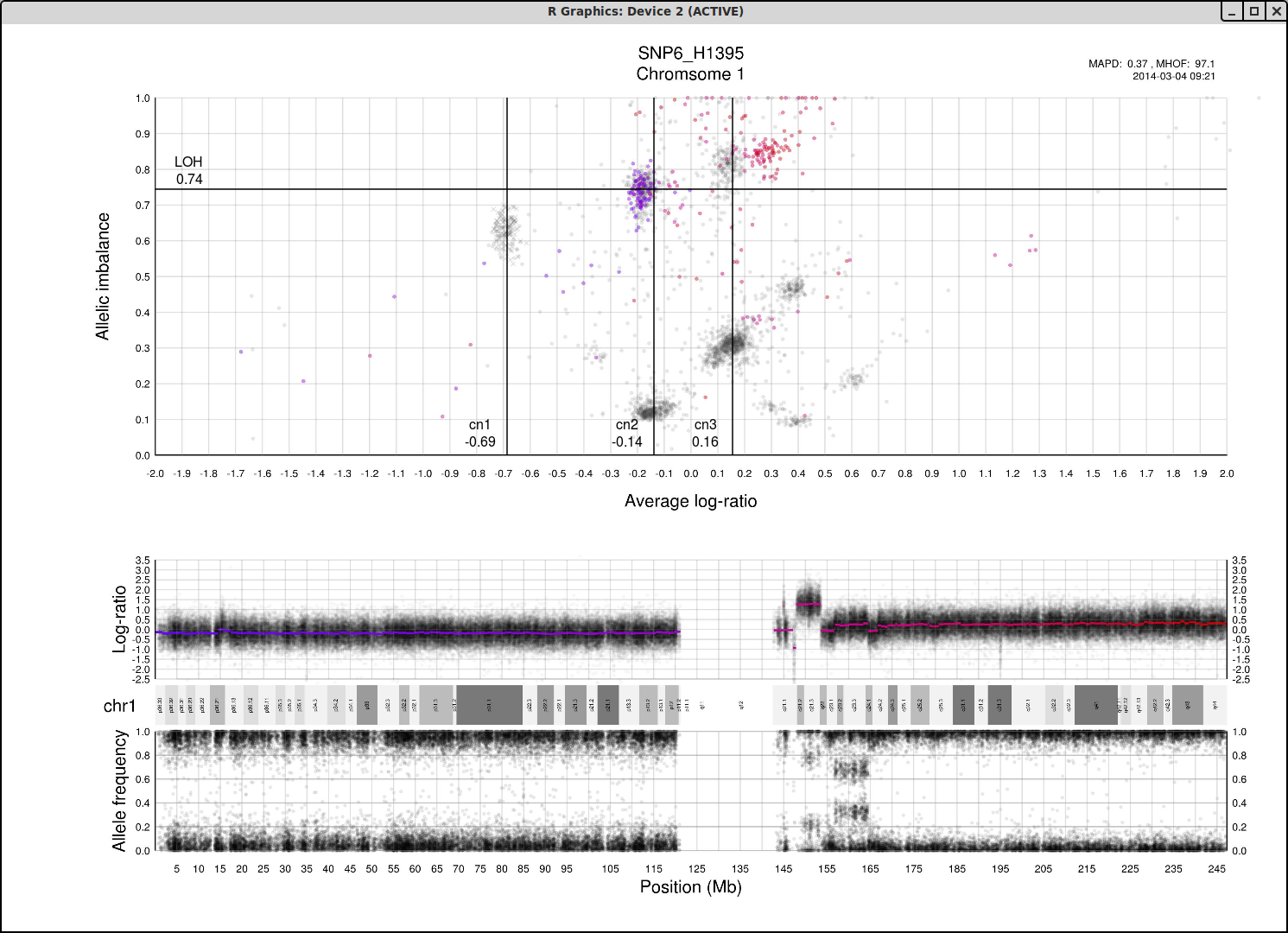
As average log-ratio increases, copy number increases. As Allelic imbalance increases, heterozygosity decreases, that is to say that clusters with high allelic imbalance will be homozygous.

What do we expect a hypothetical plots arrangement of clusters to look like? The average ploidy of the sample will be 0 on average log-ratio axis as it is normalized. The sample may be highly rearranged but quite often this is a starting point for finding copy number 2 or copy number 3. As there will be less reads covering copy number 1 in the sample than higher copy numbers and copy number 1 cannot have different allele constitutions, by its very nature of being one allele, copy number 1 will be represented by a single cluster far to the left on average log-ratio axis when compared to the other clusters.

What if we do not have any copy number 1 in the sample? Then perhaps the far left of the plot will be occupied by two clusters, indicating the homozygous, LOH, and heterozygous states of copy number 2. It then stands to reason that the next cluster we will encounter, again; moving from left to right on average log-ratio axis, will be copy number 3.
In the same way we would expect copy number 2 to follow copy number 1 in the previous scenario. Note also that the lowest allelic imbalance of copy number 3 MUST be higher than the lowest allelic imbalance of copy number 2 as copy number 2 can have one of each allele while copy number 3 must, at lowest allelic imbalance, have two of one allele and one of the other.
The X chromosome is shown as "X"'s instead of gradient circles and may also be far left, do not let it disturb your assessment of copy number levels as it can be misleading.

It is with reasoning such as this, looking at the plot and how the clusters are arranged and what cluster constitutions are physically possible, that we can determine the allele-specific copy numbers in our sample.

Here is the topmost section of one such plot with some added bars and text for tutorial purposes. The plot shows the whole sample in grey and the chosen chromosome, not important in this guide, in red to blue gradient. From this whole sample picture you can then use the arrangement of the clustered areas to estimate copy numbers and allele-specific information.



The cn1, cn2 and cn3 arguments are the positions of copy number 1, 2 and 3 on the "Average log-ratio" axis. In this example cn2 is ~ -0.15. You need only provide any two of these values later for TAPS_call().
The loh argument is the position of homozygous copy number 2 (LOH) on the "Allelic imbalance" axis. In this example loh is ~ 0.75.

We have developed two functions, TAPS_estimate() and TAPS_click(), that you can use if you do not want to fill SampleData.csv by hand. This is especially useful if you are running multiple samples. We would recommend that you always use TAPS_click().

TAPS_estimate()

TAPS_estimate() attempts to estimate the SampleData.csv arguments for all samples in the current working directory. This information is hard to automate therefore it will not always do so correctly, but it will still simplify the process when running TAPS_click() where you can either choose to accept TAPS_estimates() evaluation or redo it yourself.

TAPS_click()

TAPS_click() does NOT work with Rstudio. R must be started from the commandline.

TAPS_click() launches a GUI for sample by sample interpretation of parameters. Much like TAPS_estimate(), the output of TAPS_click() is in the form of inserting arguments for each sample into SampleData.csv. If TAPS_estimate() has been executed prior to TAPS_click(), the first thing shown will be TAPS_estimates() interpretation, see plot 1 below. At this stage you will be prompted by menu 1 and you will be given the choice to accept or redo the interpretation.

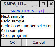
Menu 1, giving you choices to go to next sample (accept current estimates), redo the chromosome selection and interpretation of copy numbers of this sample, redo only the interpretation of copy numbers, skip the sample or close the program.

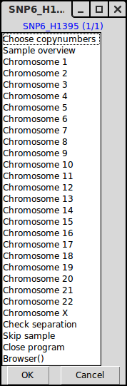
Menu 2, choose to enter an interpretation of the copy numbers or look at a specific chromosome.

• 

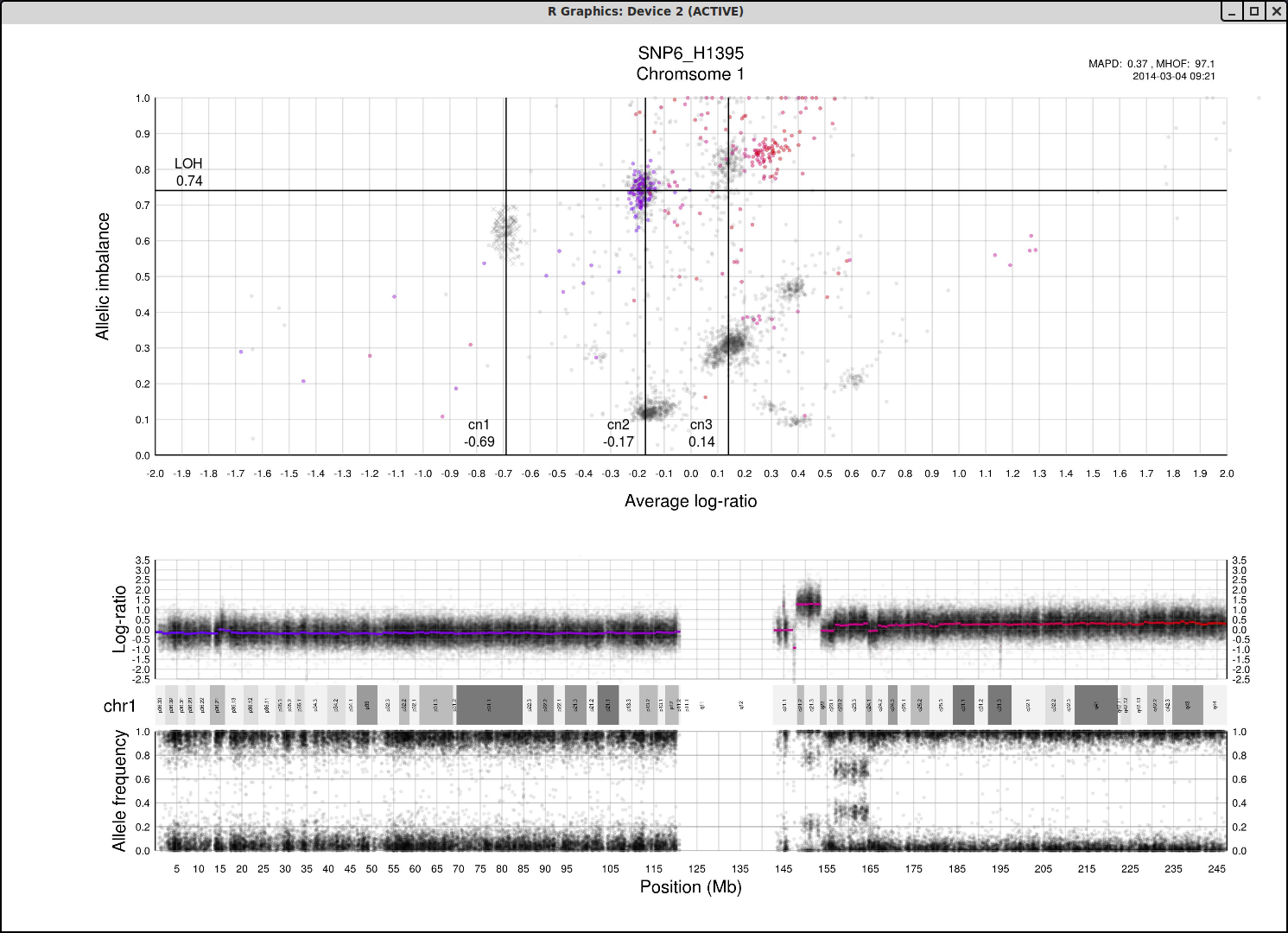
  Plot 1, TAPS_estimates() estimation of parameters for a sample. In this case the estimation is correct.

• 

  Plot 2, here we have chosen to perform copy number selection and have been prompted to identify via mouseclick the location of CN1.

• 

  Plot 3, TAPS_click() continues to prompt for input until completion. Here we have identified CN2.

• 

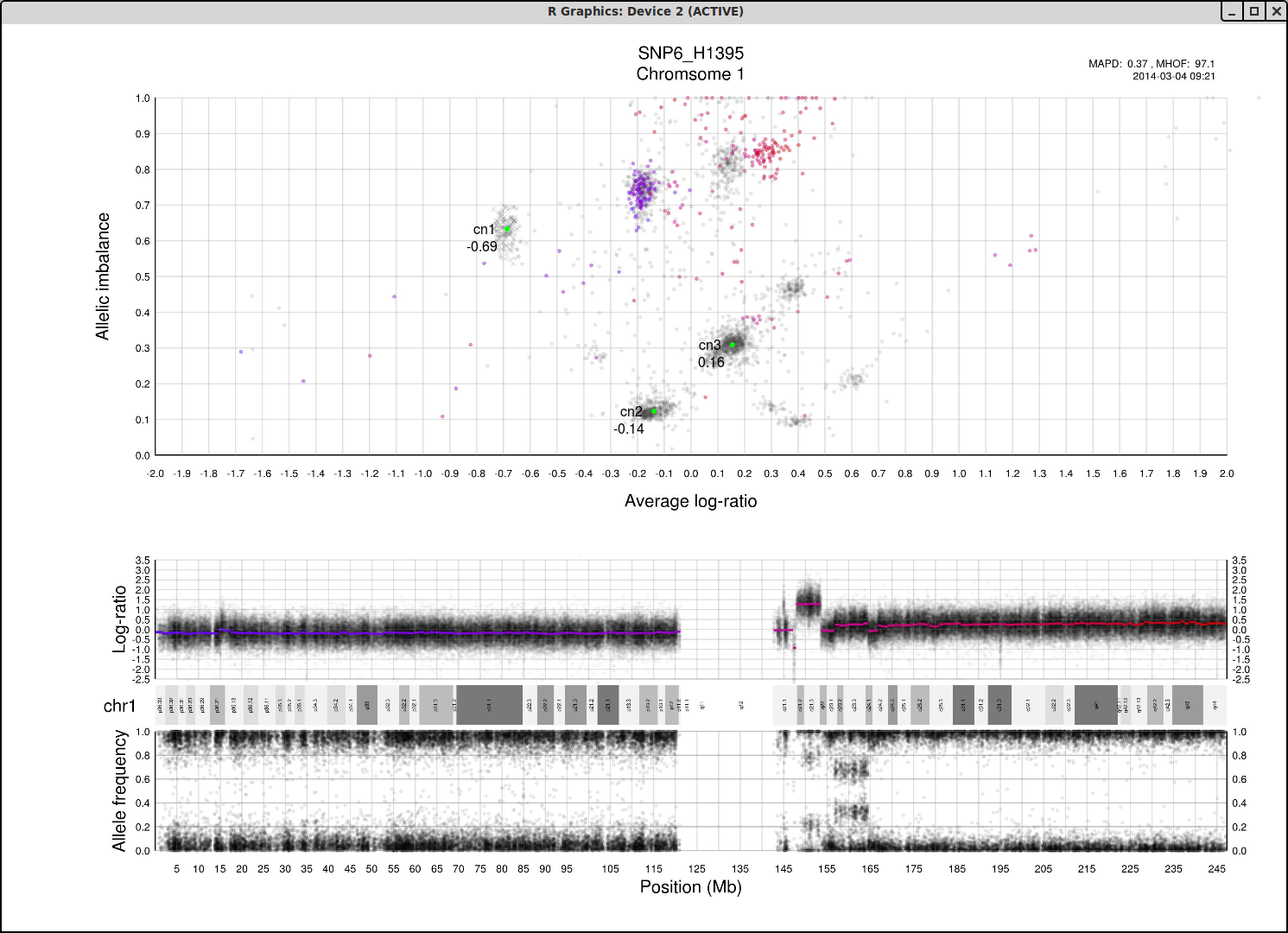
  Plot 4, CN3.

• 

  Plot 5, CN2LOH. The position of copy number 2 which has loss of heterozygosity. Located directly above copy number 2.

• 

  Plot 6, your new updated copy number interpretation. You will once again be prompted with menu 1 to move on to next sample etc.

---

TAPS_call()

The function TAPS_call() uses the relationship between log-ratio and allelic imbalance to assign copy number and allele ratio for each segment.

TAPS_plot() must have been executed before TAPS_call() can be. This is because the .Rdata files generated during TAPS_plot() will be automatically read by TAPS_call() and you need to evaluate the plots generated by TAPS_plot() to be able to give TAPS_call() meaningful input.

TAPS_call() has "directory" as its main argument, the parameters are read from the file "SampleData.csv".

An example call to TAPS_call(), where "mainsamplefolder" contains SampleData.csv:

	TAPS_call(directory="path/to/mainsamplefolder")

After running TAPS_call() you will have an additional set of plots in the sample folders which includes your analysis of the plots.

In the results tab we will look at interpreting the data. If you get any errors that you can't solve, please send us an email and we will get back to you as soon as possible!

Plots of TAPS_plot()

After running TAPS_plot() you should have chromosomal plots and an overview plot in your sample folder.

For information regarding allelic imbalance and average log-ratio click here.

Overview plot

Top half of the plot

All the possible chromosomes plotted for allelic imbalance versus average log-ratio. The colored segments represent a specific chromosome while the grey is the rest of the sample. If you look closely there are three grey bars in each plot. The middle bar is located at 0 average log-ratio, the ploidy of the sample.

Bottom half of the plot

Log-ratio, cytoband and allele frequency information for each chromosome. The colored segments in log-ratio correspond to the chromosome specific colored segments seen in the top part of the plot.

Chromosomal plots

Top half of the plot

The clusters in the plot display regions of certain allelic constitution and copy number. The copy number increases along the average log-ratio axis while paternal/maternal allele ratio becomes less balanced along the allelic imbalance axis.

The chromosome in question is colored against a background of the rest of the sample in grey. A colored circles gradient correlates with its segments position, seen in log-ratio, on the chromosome.
The circles are semi-transparent so a darker hue, both for colored and grey, indicate a greater amount of genomic content in that region.

The interpretation of this part of the plot especially in allele-specific copy numbers is the input for TAPS_call() and has been stated in TAPS execution tab.

Quoted here for your convenience:

"Lets take a look at the structure and placement of clusters on the whole genome plot.

As average log-ratio increases, copy numbers increases. As allelic imbalance increases, heterozygosity decreases, that is to say that clusters with high allelic imbalance will be homozygous.

What do we expect a hypothetical plots arrangement of clusters to look like? The average ploidy of the sample will be 0 on average log-ratio axis as it is normalized. The sample may be highly rearranged but quite often this is a starting point for finding copynumber 2 or copynumber 3. As there will be less reads covering copynumber 1 in the sample than higher copynumbers and copynumber 1 cannot have different allele constitutions, by its very nature of being one allele, copynumber 1 will be represented by a single cluster far to the left on average log-ratio axis when compared to the other clusters.

So what if we do not have any copynumber 1 in the sample? Then perhaps the far left of the plot will be occupied by two clusters, indicating the homozygous, LOH, and heterozygous states of copynumber 2. It then stands to reason that the next cluster we will encounter, again; moving from left to right on average log-ratio axis, will be copynumber 3.
In the same way we would expect copynumber 2 to follow copynumber 1 in the previous scenario. Note also that the lowest allelic imbalance of copynumber 3 MUST be higher than the lowest allelic imbalance of copynumber 2 as copynumber 2 can have one of each allele while copynumber 3 must, at lowest allelic imbalance, have two of one allele and one of the other.
The X chromosome is shown as "X"'s instead of gradient circles and may also be far left, do not let it disturb your assessment of copynumber levels as it can be misleading.

It is with reasoning such as this, looking at the plot and how the clusters are arranged and what cluster constitutions are physically possible, that we can determine the allele-specific copynumbers in our sample."

Bottom half of the plot

Log-ratio, cytoband and allele frequency information for the selected chromosome. The colored segments in log-ratio correspond directly to the colored segments seen in the top part of the plot.

Higher copy numbers will have a higher log-ratio.

Allele frequencies detected will vary depending on the allelic constitution of a segment of a chromosome. Seen here in the very frist part of the chromosome, between 0-30mb approximately, where the sample is copy number 2 with loss of heterozygosity. This means there is no variation in the allele constitution for that segment. Looking on at the rest of the chromosome in question it is copy number 3 with 2 of one allele and 1 of the other. This is shown in the banded structure, given by presence of more than one option, of allele frequency as well.

---

Plots of TAPS_call()

TAPS_call() generates you interpretation, as specified in execution tab, of the allele-specific copy numbers in the sample. It generates chromosomal plots similar to the ones of TAPS_plot() but additionally specifies total and minor copy numbers of segments. It also generates a quick "check" overview of the sample with all allele-specific copy numbers specified.

Check

This plot, arbitrarily named "check", is not chromosome specific and shows the complete tumor sample with assigned tags for copy number and allele content, much like the explanatory picture seen previously but with text describing the copy numbers and allele ratios of the segments rather than purple and green bars.

1m0 is copy number 1, homozygous.
2m1 is copy number 2, heterozygous.
2m0 is copy number 2, homozygous.
3m1 is copy number 3, heterozygous.
3m0 is copy number 3, homozygous.
And so on.

If the texts showing the approximate positions of the allele-specific copy numbers seem missplaced you may want to try to improve, or tweak, your input values in SampleData.txt, the parameters used by TAPS_call().

Chromosomal plots with total and minor copynumbers

The "by chromosome" plots generated by TAPS_call() are quite similar to the chromosomal plots generated by TAPS_plot() with the addition that they now include your allele-specific copy number analysis to display total and minor copy numbers.

Left half of the plot

The whole sample with the current chromosomes, in this example chromosome 7, segments colored from blue to red. The X chromosome is shown as X's. The size of the circles vary with length of segment, larger for larger segments. Allele-specific copy numbers of the different clusters, 1m0, 2m1 etc, are shown for quick interpretation.

Right half of the plot

Farthest up we see the total copy number, colored, and minor copy number, grey, of a segment. If a segments total copy number is 3 and minor copy number is 1 then that segment of the chromosome has 1 paternal and 2 maternal OR 2 paternal and 1 maternal copies.
Another example; if a segments total copy number is 2 and minor copy number is 0 then that segment of the chromosome has 2 paternal OR 2 maternal copies.

Below that we see the same three plots of log-ratio, cytoband information and allele frequency as seen above in chromosomal TAPS_plot() plots. Notice that all four of the plots on the right side have the position on the chromsome in question as their x axis.

---

TAPS_Region()

TAPS_region() is used to take a closer look at a specific region of the genome. Additionally it displays known genes of this region. The current gene list is the UCSC known gene list, hg18 & hg19, of march 2014.

Usage:

     TAPS_region(directory=NULL,chr,region,hg18=F)
     
Arguments:

directory: Default is getwd().Directory must contain TAPS_plot_output.Rdata,
          an output from TAPS_plot(), which contains all information that TAPS_region() needs.

     chr: Supply the chromosome you wish to look at. ex: chr=1

  region: The region of the chromosome you are interested in. ex:
          region=10000000:13000000

    hg18: Default is FALSE, meaning the hg19 known gene list will be
          used. If TRUE the hg18 known gene list is used.

Now lets take a look at an example plot of region 18000000-23000000 of chromosome 1 for sample 6295.

TAPS_region(chr=1,region=18000000:23000000)

Most of the content of the plot has been discussed above. Unique to the TAPS_region() output is the red "Selected region" marker on the whole chromosome view, which spans logRatio, cytoband information and allele frequency. This selected region is then shown in the bottom half of the plot, with an additional row of known gene information.
Notice that you chose the size of the region. Larger regions will have gene information that is hard to discern whereas very small regions might seem void of content. About 5 million basepairs, as seen here, or smaller is recommended.

For more background information please contact us!